Galaxy Simulator Parameters Defined
Quick Links to Specific Definitions
Potential Solver Methods
The simulator uses potentials of the form
Φtotal = Φbg+ Φsg
to derive the force on the particles, where Φbg is an
imposed background potential and Φsg is the potential
due to the self-gravity of the particles. Self-gravity can be turned
on or off (as can the background potential) and integrated by
selecting the desired potential solver method.
No Self Gravity: This option turns
off self-gravity so particle motion may be evaluated using only a
background potential.
Direct Force Summation: This method
finds the acceleration on each particle directly by adding up the
accelerations due to all the other particles individually according
to
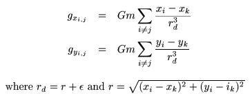
This is a very inefficient and costly
integration method; it should only be used when evaluating a small number of particles.
Fourier Method: The potential can
be found more efficiently using the Fourier method. This method uses
Fourier transforms on a grid of
Nx x Ny cells to determine the
potential and mass density in each cell. The complete method is
complicated, but is much more efficient for determining the potential
due to a large number of bodies and should be used instead of direct
force summation unless only a small number of particles are involved.
For a more complete description of this method see the paper written by the original authors of the simulator.
Potential
Types
The force, and therefore the acceleration, experienced by a particle is derived from the potential field in which the particle resides: F = -∇Φ. The simulator provides many models for the background potential.
No Background Potential: This option
turns off the background potential so that particle trajectories may be evolved using only self-gravity.
Power Law Potential: The simulator
uses a power law
potential of the form
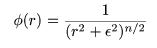 ,
,
where ε is a smoothing parameter and is input as param2; the value of n is given by
param1. n = 1 provides a Keplerian potential.
Time Dependent Bar Potential: The time
dependent and independent bar potentials used by the simulator are logarithmic potentials of
the form
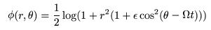
The variable ε is a parameter which scales the effect of the bar and is input as param1. Ω is the angular frequency and is given by param2.
Harmonic Potential: This
option is a harmonic
potential is of the form
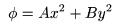
In the simulator, the scaling
factors A and B are input as param1 = A and param2 = B. These scaling factors determine the relative strength of the field in x and y.
Isochrone Potential: The
isochrone potential is a reasonable approximation to a disc galaxy
with roughly constant density near the center and the density going to
zero at larger radii. The simulator uses the form
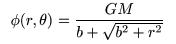
The variable b is given by param1 and the disc mass M is param2.
Homogeneous Sphere
Potential: The homogeneous sphere simulates the
potential due to a sphere of uniform density. This is a practical
approximation to a large massive central object or the potential due
to a halo near the center of an otherwise thin disc galaxy. The form
used is
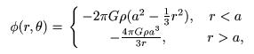
The sphere radius a is input as param1, and the sphere density ρ is param2.
"Galaxy" Potential: The galaxy potential is actually a combination of Keplerian, homogeneous sphere and logarithmic potentials as described above. This combination is designed to model a large disc galaxy with a halo and central compact object. For this potential the input parameters param1 and param2 are not used.
Integration Methods
Finding each particle's position and velocity for each timestep
requires knowing the particle's acceleration and initial conditions
for that timestep. The acceleration is determined using the potential at
each location according to
 ,
,
and similarly for the y
direction, noting that the simulator normalizes
all particle masses to unity. From there, the positions and
velocities are found using one of the available numerical integration
schemes. For in-depth detail of these methods, with computer code, see
W.H. Press, S.A. Teukolsky, W.T. Vetterling, and B.P. Flannery,
Numerical Recipes in C: The Art of Scientific Computing, 2nd
edition, 1997. Additionally, the graphical representations of the
integration methods were obtained from http://www.physics.drexel.edu/courses/CompPhys/Integrators/
prepeared by Steve
McMillan at Drexel University.
Euler Method: The Euler
integration scheme is the simplest available in the simulator. It is computationally
cheap, but because it is only first order its error term is second
order in the timestep, making it a relatively inaccurate integration
method. A graphical representation along with the formulae is shown below.
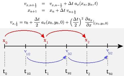
| Leapfrog Method:
The Leapfrog integration method is only slightly higher in
computational cost than the Euler method, but it's error term is third
order. As can be seen in the diagram and formulae, this method uses
the derivatives at the midpoint of each step. This only requires one
additional step to be taken in order to move the velocity a half
step ahead of the position. Because of its better accuracy while
still keeping the simulation generation time relatively low the
Leapfrog method is the default integration scheme.
| 
|
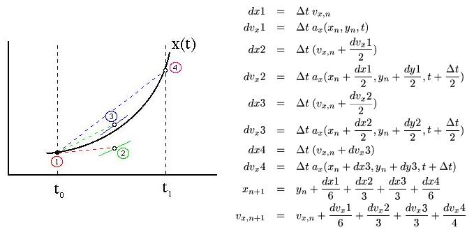
Midpoint Method: The
Midpoint method is similar to the Euler method in that it starts by
taking an Euler "trial step." It then uses the values
obtained by the trial step to take real steps according to the
formulae shown. This method also has an error term that is third
order, but it is more computationally expensive than the Leapfrog
method. It is important, however, since it is more easily generalized
to the much more accurate (and expensive) Runge-Kutta and Cash-Karp schemes.
Runge-Kutta Method: The
Runge-Kutta method is a fourth order integration technique similar to an
expanded Midpoint scheme. This method takes four trial steps and uses
their weighted average to advance the particle according to the
formulae shown below. It is highly accurate, having a fifth order
error term, but it is computationally expensive.
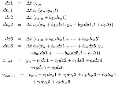
| Cash-Karp Method: The
Cash-Karp method is basically the same as a fifth order Runge-Kutta
scheme. It uses various constants found by Cash and Karp (see
Numerical Recipes, 2nd edition) in the formulae shown. This
is the most accurate integration technique available on the simulator,
having a sixth order error term, but it is less practicle because of
its enormously high cost in computational time.
| 
|
Self Gravity Leapfrog Method:
Other Simulator Parameters
Time Duration: This input gives the total time duration of the simulation.
Timestep: The timestep sets the time interval Δt used in the integration scheme.
Image Frequency: The image frequency tells the simulator how often to "dump" the simulation data in numbers of timesteps. Each of these dumps is used to create a frame in the final movie, so the number of frames that will be present is given by the time duration divided by the product of the timestep and image frequency.
Alpha: The parameter "Alpha" is a measure of dispersion in a Gaussian surface density distribution. The simulator uses a surface density of the form
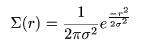
Alpha provides the value of the variable σ in the above formula.
Other Stuff
Students working on the simulators available in the Digital Demo Room
participate in the "Research Experience for Undergraduates",
or REU, program in the Physics Department of the University of
Illinois. The students give presentations on their projects and also
write a scientific paper. The paper for the Thin Disc Galaxy
simulator, which was built by Scott Olsson and Geert Vrijsen during the 2001 REU program,
is available here for anyone interested in seeing the development of
this pedagogical project.
Return to the simulator!