The Digital Demo Room
One-Dimensional Hydrodynamics Simulator
Behind the Simulator: An Explanation
The Image Produced by the Simulator
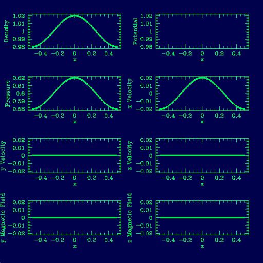
| The simulator produces a series of images in sequential timesteps
which are then assembled into an animated movie file to show the
evolution of the wave over the length of time under evaluation.
Each image file shows eight plots. Each plot represents a different
property of the wave or its medium and shows how its value changes
over a one-dimensional distance for that timestep. The
first frame (like the one shown) will show the wave under its initial
equilibrium conditions. The simulator will then introduce a
perturbation and the following frames show how that perturbation
affects the wave.
The eight properties are, in order from left to right, top to bottom,
density, potential, pressure, x velocity, y velocity, z velocity, y
magnetic field and z magnetic field. Which properties exhibit
variations depends on the type of wave being propagated; for instance,
this image illustrates the first frame of a sound wave mpeg in a
medium with no magnetic fields or background potentials (such as
gravity). In this case only the density, pressure and x velocity
plots show any variance.
OK, this is supposed to be a one-dimensional simulation, so why are
there plots for velocities in the y and z directions? Good question!
For this simulator, "one-dimensional" refers to the wave
vector k of the wave being propagated. However, the presence
of magnetic fields will cause transverse motion in a charged medium, so plots are included to show the
velocities of the transverse waves in the y and z directions caused by these fields.
Obviously, the y and z velocity plots will only exhibit motion when a
non-zero magnetic field value has been included in the simulation.
|
| Sound Wave at Equilibrium
|
|
The Waves
Linear Waves:
To create a linear wave, the equations of motion for a fluid wave have been
"linearized;" ie, in solving the equations variables higher
than first order have been dropped. Several different linear waves,
both hydrodynamic and magnetohydrodynamic (ie, influenced or produced by magnetic fields), are available in the simulator:
Alfven Wave:
Alfven waves result from oscillations caused by the transverse motion of
magnetic induction lines. Magnetic tension provides a restoring force
to the induction lines to bring them back to a straight line,
producing the transverse Alfven waves. The simulator introduces a perturbation into the magnetic field and plots the resulting disturbance.
Entropy Wave:
Entropy waves, which can be either hydrodynamic or
magnetohydrodynamic, are compressional waves (ie, fluctuations in
pressure and density) in which the internal energy and velocity
remains constant (unless a gravitational potential is introduced).
Fast/Slow Waves:
Sound Wave:
Sounds waves, like entropy waves, are hydrodynamic compressional waves
that propagate a fluctuation in pressure and density. Unlike entropy
waves, the internal energy of sound waves varies while entropy remains constant.
Shock Tubes:
A shock tube is less a wave than it is a moving wall of force. The shock
itself is a discontinuity, having an instantaneous jump in fluid
pressure, density and velocity on either side of the shock. The
simulator therefore requests values for these parameters both on the
left and right sides of the shock as part of the initial conditions.
The default conditions used by the simulator match the Sod
hydrodynamic shock tube problem described by Brio & Wu (see Journal of
Computational Physics, 1988, volume 75, page 400).
The Parameters
Two basic types of parameters are used in the One-Dimensional
Hydrodynamics simulator: physical and computational. The parameters
that the simulator will request from the user varies based on the type of
wave selected and the level of knowledge the user chooses. In some
cases a parameter's value may be hidden or unnecessary for the
particular simulation. Default values for all parameters are provided.
Computational Parameters:
Computational parameters are used by the simulator to perform
calculations and also to set up conditions and ranges on the simulation.
Boundary Conditions:
The boundary conditions tell the simulator what to do with the wave at
the edges of the plot. Three options are available: periodic,
reflecting and standard. Periodic boundary conditions cause the wave
to appear on the opposite side of the graph after it moves past a
boundary. With reflecting conditions the wave will "bounce
back" from the edges (careful - this condition may cause the wave
to "interfere" with itself). Under standard conditions the
wave will simply move into a "ghost zone" after passing a boundary.
Courant Number:
The Courant number helps determine the size of dt, or the magnitude of
the timestep between frames. A larger value of the Courant number
causes a larger value in dt, and therefore less frames in the final simulation.
Dumping Frequency:
The dumping frequency parameter tells the simulator how often to
create an image file. Smaller values result in larger numbers of
images since the dumping frequency is calculated as a multiple of the
wave frequency. A value of 0.1 will result in 10 images for every
wave oscillation, and will therefore require additional computation
time and produce a larger mpeg file.
Integration Time:
The integration time parameter determines the length of the time scale
run by the simulator, and, therefore, the number of frames in the
resulting movie file. A larger value for the integration time will
require a longer wait as the simulator performs computations and will
also result in a larger mpeg. Users with slow internet connections
may want to opt for smaller integration times.
Numerical Resolution:
The numerical resolution determines the "smoothness" of the
wave by setting the number of points plotted. The distance scale is
divided by the numerical resolution to calculate dx, or the amount of change in
"x", for each point plotted. The image above was plotted
with a numerical resolution of 128, which is a good default value.
Larger values for this parameter greatly increase the length of time
required to perform calculations.
Physical Parameters:
Physical parameters determine the properties of the wave and medium
being evaluated.
Adiabatic Index:
In an adiabatic process the entropy of each fluid particle remains
constant and therefore no heat exchange occurs between different
fluid elements. The adiabatic index, denoted γ, describes the
specific heat ratios of fluid elements in the Poisson adiabatic
formula: pVγ=constant. The typical value for this parameter is 5/3.
Amplitude:
The amplitude parameter determines the maximum and minimum height of
the wave. The simulator associates the amplitude value with one of
the physical properties of the wave used in its eigenvector and may be
different depending on the type of wave selected. For instance, the
amplitude of a sound wave determines the maximum and minimum values of
the wave velocity.
Artificial Viscosity:
Only an ideal fluid or gas will move with no energy lost to the
irreversible transfer of momentum from internal friction between fluid
elements with differing velocities. The artificial viscosity
determines the extent to which this energy is lost during fluid flow.
Density:
The density defines the number of fluid particles in a set volume (in
this case a volume containing a unit mass of fluid) or the "thickness" of the fluid element.
Gravitational Potential:
On a small scale, gravity has a negligible effect in the fluid
equations of motion. However, on large scales such as those found in
astrophysical applications gravitational potential can have a dramatic
effect. The gravitational potential is given by the Laplacian
equation: ∇2Φ = 4πGρ.
Pressure:
Pressure is the amount of force exerted on the fluid by the wave.
Magnetic Fields:
Magnetic fields can have a dramatic effect on a wave composed of
charged particles, and vice versa. A non-zero value for the magnetic field
will affect the wave's velocity according to the "right-hand
rule," causing transverse motion.
Wave Vector:
The wave vector defines the quantum energy state of the wave, and must be an
integer value of one or higher. Any decimal inputs for the wave
vector parameter will automatically be adjusted to the next lowest
integer energy state by the simulator.
Wave Velocities:
The velocity tells the direction and speed of the wave. Since this
simulator is one-dimensional, all wave velocities will be in the
"x" direction unless magnetic field values are included that
cause transverse motion in the wave. Any components of the wave
velocity in the "y" or "z" directions will be
indicated by the y and z velocity plots.
Other Stuff
Students working on the simulators available in the Digital Demo Room
participate in the "Research Experience for Undergraduates",
or REU, program in the Physics Department of the University of
Illinois. The students give presentations on their projects at the
midpoint and end of the summer research program and also write a
paper. The presentations and paper for the One-Dimensional
Hydrodynamic simulator, which was built by Conley "Lee" Ditsworth during the 2002 REU program,
are available here for anyone interested in seeing the development of this pedagogical project:
Midpoint Presentation
Final Presentation
Final Paper
Return to the simulator!