Digital Demo Room
Stellar Structure and Evolution Simulator
Visualization Methods
Stellar Evolution Code
| 1 | - | Main Sequence Star |
| 2 | - | Hertzsprung Gap |
| 3 | - | First Giant Branch |
| 4 | - | Core Helium Burning |
| 5 | - | First Asymptotic Giant Branch |
| 6 | - | Second Asymptotic Giant Branch |
| 7 | - | Main Sequence Naked Helium Star |
| 8 | - | Hertzsprung Gap Naked Helium Star |
| 9 | - | Giant Branch Naked Helium Star |
| 10 | - | Helium White Dwarf |
| 11 | - | Carbon/Oxygen White Dwarf |
| 12 | - | Oxygen/Neon White Dwarf |
| 13 | - | Neutron Star |
| 14 | - | Black Hole |
For each class, an analytic formula is known that fits data from a comprehensive stellar evolution code. This formula is a function of initial mass, metallicity, and time. Binary stars and specific kinds of mass loss are incorporated in SSE, but are not used in the DDR. The SSE formula returns current total mass, core mass, luminosity, temperature, radius, and spin at every timestep for an individual star.
We limit the possible input masses to lie between 0.1 and 100 solar masses. Below about 0.1 solar masses, stars will probably not begin hydrogen fusion. It's uncertain if any stable stars with masses greater than 100 solar masses exist.
Metallicities are calculated as the log of the mass fraction of elements heavier than Helium(He) in the star, and the starting metallicity affects the subsequent evolution. The main sequence is based on stars of solar metallicity (0.02). For this reason stars created with different metallicities may not begin precisely on our main sequence. The metallicity ranges from 0.0001 to 0.03. Stars with extremely low metallicities are slightly warmer and appear to the left of the main sequence. Stars with high metallicities are cooler and appear to the right.
The formation of stars in a star cluster is determined by a stellar mass function or initial mass function (IMF). This mass function is an analytic model for determining the approximate number density of a star of a particular mass in a star cluster. Basically, it is a function that describes how many stars of which masses would exist in a cluster if every star was born at the same time. (Binney and Merrifield). The stellar mass function that we use in our simulation is known as the Scalo equations.
This IMF describes the number of stars in a stellar population within a specific differential mass range (Allen). The number of higher mass stars in a given stellar population allowed by this IMF is much smaller than number of lower mass stars. The result is that for star clusters and stellar populations which this IMF models, there should be many more low mass stars than high mass stars, and such is the case observationally.
In our simulation, we have given the user the option of choosing a number of randomly massed stars that will be generated by our code determined by the above IMF. In essence, the user has the ability to create a newly formed stellar population between any mass range he/she chooses, with masses accurately determined by the IMF, and to watch it evolve on an HR diagram. To utilize the IMF in creating these randomly generated masses, we first normalize the IMF to a peak value of 1. We then randomly generate a mass between the user's limits, and this random mass is input into the part of the IMF that corresponds to its mass. We then generate another random number, this time between 0 and 1, and we test this number. If this new number is greater than the value that we received from inputting the random mass into the IMF, we reject the random mass and we start over, generating a new random mass. If this new number is less than or equal to the IMF's output value, we keep the random mass and use it as one of the stars that goes to the final simulation. This happens many times until as many randomly massed stars as are needed have been accepted. Essentially, what we did was to generate a random mass, check its probability of existing in a stellar population with the normalized IMF, and then either reject it or keep it depending on this probability.
The stable hydrogen burning lifetime of a star can vary from a few million years for high mass stars to tens of billions of years for low mass stars. We give the user a choice of 500, 1000, or 1500 frame movies. To see the details of the evolution of both high mass stars and low mass stars in the same movie would require varying the rate that time passes. This approach would give a false sense of the relative timescales, so all of the DDR movies are in linear time. To make sure the time scale for each movie encompasses the lifetimes of all stars used, the ending time is set by the lifetime of the lowest mass star in the movie. The lifetime is defined to be the point at which the star becomes a white dwarf, neutron star or black hole. The movies show an additional fifteen percent past the longest lifetime to show cooling of the final states. This way a group of very high mass stars will only be evolved for a few million years, and with a lower final time, each frame is a smaller timestep, and different stages can be seen in detail. In order to better view these different stages, the user has the option for the stars to leave trails on the graph.
The default setting for the simulation creates all stars at the same time. This creates a very clear turn-off point on the main sequence, as higher mass stars rapidly evolve. Other options allow for multiple star creation times (having several 'starbursts'), or continous star creation. Within the continous creation, there are options for having a constant, increasing, or decreasing star creation rate. This allows simulations to be tuned to specific creation environments, such as HII regions or globular clusters.
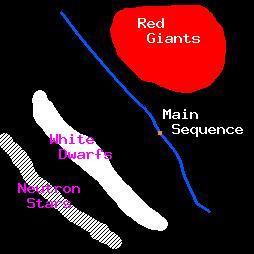
The axes of the HR diagram were chosen to highlight the evolution closest to the main sequence. The cooling of white dwarfs and neutron stars is included in the SSE code, but we felt that it was too uncertain to focus attention on. Neutron stars do not appear within the bounds of the graph. White dwarfs appear for most of their cooling phase. Black holes have no luminosity and do not appear at all. Naked helium stars are so hot, that to expand the axes to fit them on the graph would shift the attention away from the main sequence. For that reason, naked helium stars do not appear on the graph, although their supernovas still appear near the axis labels. The very highest mass stars can also briefly become too luminous to appear within the bounds of the graph.
The colors of the stars are not exact, but instructional nonetheless. Color is determined entirely by the star's temperature, but there is no exact formula to translate temperature into an RGB triplet. Blackbody peak radiation wavelength can be used as an estimate. For this simulation, six different colors were chosen and associated with specific temperature ranges. The colors were based on the colors assigned to real stars. For stars that lie outside of those specific temperature ranges, the color is interpolated in RGB between the two nearest colors. Blue is associated with main sequence high mass stars and red is associated with main sequence low mass stars and red giants. In between these colors we have light blue, white, yellow, and orange, in order of decreasing temperature.
Since temperature and luminosity can seem rather abstract to beginning students, radius data is also incorporated into the simulation for single star movies. The radius data is reconstructed from the temperature and luminosity. The formula R2 ~ L/T4 is used to calculate the star's radius at each time. The radius of a star can range from about 0.1 to 1000 times the radius of the sun, so we show a picture of a star with a radius proportional to the log base 10 of its true radius, in the appropriate color. This is shown in a separate box next to the HR diagram. This way a student can see a star expanding and contracting through its various phases.
This same box that shows the star's size also demonstrates the star's spin. An analytic approximation to the spin rate of stars is used for animation purposes, and the spin rate changes as the star evolves. However, our simulation shows the spin of the star on a different timescale than the evolution timescale. While every frame represents at least several thousand years, a typical star will complete one revolution in a matter of days. We add the spin to the simulation to show qualitatively that not only do stars spin but that the spin rate changes with radius.
Finally, an attempt is made to account for convective versus radiative surfaces. Below about 1.2 solar masses, a star's surface is convective, leading to solar flares, sun spots, and a highly unstable appearance. For high mass stars, the surface is radiative and generally thought to be quite uniform, so the picture is smoothed out. What is left after smoothing is enough to notice rotation, but not enough to indicate violent surface activity.
When a star exhausts its fuel, it can either go supernova or create a planetary nebula. This is the most dramatic event in the star's life, so it is highlighted in the simulation. When a star first forms its planetary nebula, a small circle is drawn on the HR diagram where that star was, and a picture of a planetary nebula is shown briefly in the picture box. Planetary nebulas for stars greater than about 2 solar masses (but not high enough to go supernova) have a round shape while those of lower mass stars have more elliptical or bipolar shapes. The pictures shown in the movie reflect this difference. When a star goes supernova in the movie, a small flare is drawn on the HR diagram where the star was, the HR diagram flashes for one frame, and a picture of a supernova remnant is briefly shown in the radius box. Both circles and flares fade away with time, so that a movie with many stars does not become too cluttered. A minor flaw with this visualization happens when wide ranges of star masses are used. The highest mass stars will appear to go supernova on or near the main sequence in the first few frames. This is because in these particular simulations, the time elapsed between frames is on the order of the lifetime of one the high mass stars.